A geometric interpretation of the covariance matrix
Contents
Introduction
In this article, we provide an intuitive, geometric interpretation of the covariance matrix, by exploring the relation between linear transformations and the resulting data covariance. Most textbooks explain the shape of data based on the concept of covariance matrices. Instead, we take a backwards approach and explain the concept of covariance matrices based on the shape of data.
In a previous article, we discussed the concept of variance, and provided a derivation and proof of the well known formula to estimate the sample variance. Figure 1 was used in this article to show that the standard deviation, as the square root of the variance, provides a measure of how much the data is spread across the feature space.
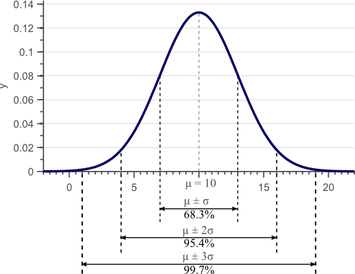
Figure 1. Gaussian density function. For normally distributed data, 68% of the samples fall within the interval defined by the mean plus and minus the standard deviation.
We showed that an unbiased estimator of the sample variance can be obtained by:
(1) ![Rendered by QuickLaTeX.com \begin{align*} \sigma_x^2 &= \frac{1}{N-1} \sum_{i=1}^N (x_i - \mu)^2\\ &= \mathbb{E}[ (x - \mathbb{E}(x)) (x - \mathbb{E}(x))]\\ &= \sigma(x,x) \end{align*}](https://www.visiondummy.com/wp-content/ql-cache/quicklatex.com-8511602375b6c3ba0dcf673f5fcdd8f9_l3.png)
However, variance can only be used to explain the spread of the data in the directions parallel to the axes of the feature space. Consider the 2D feature space shown by figure 2:
For this data, we could calculate the variance ![]() in the x-direction and the variance
in the x-direction and the variance ![]() in the y-direction. However, the horizontal spread and the vertical spread of the data does not explain the clear diagonal correlation. Figure 2 clearly shows that on average, if the x-value of a data point increases, then also the y-value increases, resulting in a positive correlation. This correlation can be captured by extending the notion of variance to what is called the ‘covariance’ of the data:
in the y-direction. However, the horizontal spread and the vertical spread of the data does not explain the clear diagonal correlation. Figure 2 clearly shows that on average, if the x-value of a data point increases, then also the y-value increases, resulting in a positive correlation. This correlation can be captured by extending the notion of variance to what is called the ‘covariance’ of the data:
(2) ![]()
For 2D data, we thus obtain ![]() ,
, ![]() ,
, ![]() and
and ![]() . These four values can be summarized in a matrix, called the covariance matrix:
. These four values can be summarized in a matrix, called the covariance matrix:
(3) ![Rendered by QuickLaTeX.com \begin{equation*} \Sigma = \begin{bmatrix} \sigma(x,x) & \sigma(x,y) \\[0.3em] \sigma(y,x) & \sigma(y,y) \\[0.3em] \end{bmatrix} \end{equation*}](https://www.visiondummy.com/wp-content/ql-cache/quicklatex.com-c3b2c0560068487dd51917cd55636781_l3.png)
If x is positively correlated with y, y is also positively correlated with x. In other words, we can state that ![]() . Therefore, the covariance matrix is always a symmetric matrix with the variances on its diagonal and the covariances off-diagonal. Two-dimensional normally distributed data is explained completely by its mean and its
. Therefore, the covariance matrix is always a symmetric matrix with the variances on its diagonal and the covariances off-diagonal. Two-dimensional normally distributed data is explained completely by its mean and its ![]() covariance matrix. Similarly, a
covariance matrix. Similarly, a ![]() covariance matrix is used to capture the spread of three-dimensional data, and a
covariance matrix is used to capture the spread of three-dimensional data, and a ![]() covariance matrix captures the spread of N-dimensional data.
covariance matrix captures the spread of N-dimensional data.
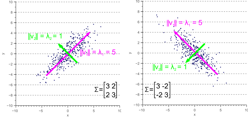
Figure 3 illustrates how the overall shape of the data defines the covariance matrix:
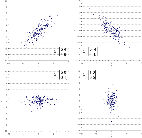
Figure 3. The covariance matrix defines the shape of the data. Diagonal spread is captured by the covariance, while axis-aligned spread is captured by the variance.
Eigendecomposition of a covariance matrix
In the next section, we will discuss how the covariance matrix can be interpreted as a linear operator that transforms white data into the data we observed. However, before diving into the technical details, it is important to gain an intuitive understanding of how eigenvectors and eigenvalues uniquely define the covariance matrix, and therefore the shape of our data.
As we saw in figure 3, the covariance matrix defines both the spread (variance), and the orientation (covariance) of our data. So, if we would like to represent the covariance matrix with a vector and its magnitude, we should simply try to find the vector that points into the direction of the largest spread of the data, and whose magnitude equals the spread (variance) in this direction.
If we define this vector as ![]() , then the projection of our data
, then the projection of our data ![]() onto this vector is obtained as
onto this vector is obtained as ![]() , and the variance of the projected data is
, and the variance of the projected data is ![]() . Since we are looking for the vector
. Since we are looking for the vector ![]() that points into the direction of the largest variance, we should choose its components such that the covariance matrix
that points into the direction of the largest variance, we should choose its components such that the covariance matrix ![]() of the projected data is as large as possible. Maximizing any function of the form
of the projected data is as large as possible. Maximizing any function of the form ![]() with respect to
with respect to ![]() , where
, where ![]() is a normalized unit vector, can be formulated as a so called Rayleigh Quotient. The maximum of such a Rayleigh Quotient is obtained by setting
is a normalized unit vector, can be formulated as a so called Rayleigh Quotient. The maximum of such a Rayleigh Quotient is obtained by setting ![]() equal to the largest eigenvector of matrix
equal to the largest eigenvector of matrix ![]() .
.
In other words, the largest eigenvector of the covariance matrix always points into the direction of the largest variance of the data, and the magnitude of this vector equals the corresponding eigenvalue. The second largest eigenvector is always orthogonal to the largest eigenvector, and points into the direction of the second largest spread of the data.
Now let’s have a look at some examples. In an earlier article we saw that a linear transformation matrix ![]() is completely defined by its eigenvectors and eigenvalues. Applied to the covariance matrix, this means that:
is completely defined by its eigenvectors and eigenvalues. Applied to the covariance matrix, this means that:
(4) ![]()
where ![]() is an eigenvector of
is an eigenvector of ![]() , and
, and ![]() is the corresponding eigenvalue.
is the corresponding eigenvalue.
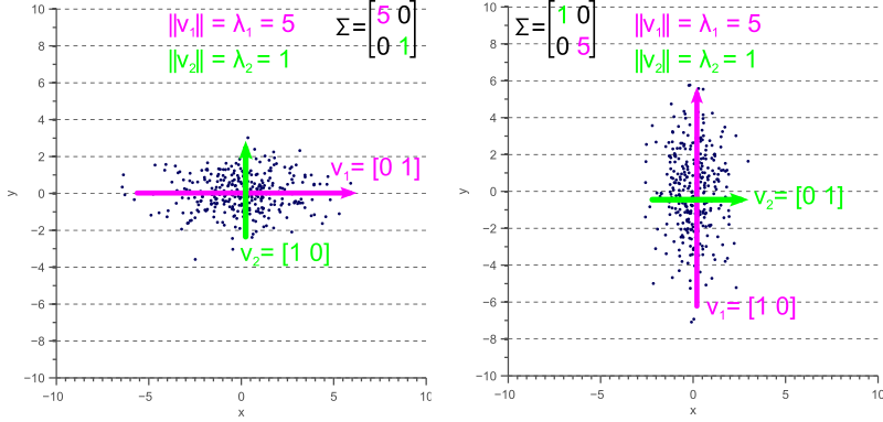
If the covariance matrix of our data is a diagonal matrix, such that the covariances are zero, then this means that the variances must be equal to the eigenvalues ![]() . This is illustrated by figure 4, where the eigenvectors are shown in green and magenta, and where the eigenvalues clearly equal the variance components of the covariance matrix.
. This is illustrated by figure 4, where the eigenvectors are shown in green and magenta, and where the eigenvalues clearly equal the variance components of the covariance matrix.
However, if the covariance matrix is not diagonal, such that the covariances are not zero, then the situation is a little more complicated. The eigenvalues still represent the variance magnitude in the direction of the largest spread of the data, and the variance components of the covariance matrix still represent the variance magnitude in the direction of the x-axis and y-axis. But since the data is not axis aligned, these values are not the same anymore as shown by figure 5.
By comparing figure 5 with figure 4, it becomes clear that the eigenvalues represent the variance of the data along the eigenvector directions, whereas the variance components of the covariance matrix represent the spread along the axes. If there are no covariances, then both values are equal.
Covariance matrix as a linear transformation
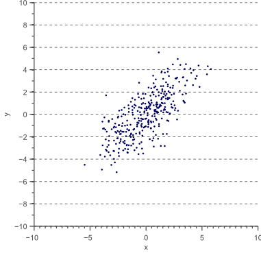
Now let’s forget about covariance matrices for a moment. Each of the examples in figure 3 can simply be considered to be a linearly transformed instance of figure 6:
Let the data shown by figure 6 be ![]() , then each of the examples shown by figure 3 can be obtained by linearly transforming
, then each of the examples shown by figure 3 can be obtained by linearly transforming ![]() :
:
(5) ![]()
where ![]() is a transformation matrix consisting of a rotation matrix
is a transformation matrix consisting of a rotation matrix ![]() and a scaling matrix
and a scaling matrix ![]() :
:
(6) ![]()
These matrices are defined as:
(7) ![Rendered by QuickLaTeX.com \begin{equation*} R = \begin{bmatrix} \cos(\theta) & -\sin(\theta) \\[0.3em] \sin(\theta) & \cos(\theta) \end{bmatrix} \end{equation*}](https://www.visiondummy.com/wp-content/ql-cache/quicklatex.com-78bf053271a867c2d5b7c2b30d3e7924_l3.png)
where ![]() is the rotation angle, and:
is the rotation angle, and:
(8) ![Rendered by QuickLaTeX.com \begin{equation*} S = \begin{bmatrix} s_x & 0 \\[0.3em] 0 & s_y \end{bmatrix} \end{equation*}](https://www.visiondummy.com/wp-content/ql-cache/quicklatex.com-0756bebe1440213107fea1005e1a655b_l3.png)
where ![]() and
and ![]() are the scaling factors in the x direction and the y direction respectively.
are the scaling factors in the x direction and the y direction respectively.
In the following paragraphs, we will discuss the relation between the covariance matrix ![]() , and the linear transformation matrix
, and the linear transformation matrix ![]() .
.
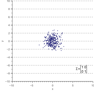
Let’s start with unscaled (scale equals 1) and unrotated data. In statistics this is often refered to as ‘white data’ because its samples are drawn from a standard normal distribution and therefore correspond to white (uncorrelated) noise:
The covariance matrix of this ‘white’ data equals the identity matrix, such that the variances and standard deviations equal 1 and the covariance equals zero:
(9) ![Rendered by QuickLaTeX.com \begin{equation*} \Sigma = \begin{bmatrix} \sigma_x^2 & 0 \\[0.3em] 0 & \sigma_y^2 \\ \end{bmatrix} = \begin{bmatrix} 1 & 0 \\[0.3em] 0 & 1 \\ \end{bmatrix} \end{equation*}](https://www.visiondummy.com/wp-content/ql-cache/quicklatex.com-22cfcbfd49a80711b48bee89d0ac5e9e_l3.png)
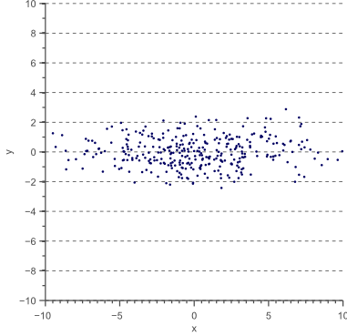
Now let’s scale the data in the x-direction with a factor 4:
(10) ![Rendered by QuickLaTeX.com \begin{equation*} D' = \begin{bmatrix} 4 & 0 \\[0.3em] 0 & 1 \\ \end{bmatrix} \, D \end{equation*}](https://www.visiondummy.com/wp-content/ql-cache/quicklatex.com-93925ded582a8e859f4efd17c75d7dc9_l3.png)
The data ![]() now looks as follows:
now looks as follows:
The covariance matrix ![]() of
of ![]() is now:
is now:
(11) ![Rendered by QuickLaTeX.com \begin{equation*} \Sigma' = \begin{bmatrix} \sigma_x^2 & 0 \\[0.3em] 0 & \sigma_y^2 \\ \end{bmatrix} = \begin{bmatrix} 16 & 0 \\[0.3em] 0 & 1 \\ \end{bmatrix} \end{equation*}](https://www.visiondummy.com/wp-content/ql-cache/quicklatex.com-b17970f14e6400c5fc20c4b9c069abfd_l3.png)
Thus, the covariance matrix ![]() of the resulting data
of the resulting data ![]() is related to the linear transformation
is related to the linear transformation ![]() that is applied to the original data as follows:
that is applied to the original data as follows: ![]() , where
, where
(12) ![Rendered by QuickLaTeX.com \begin{equation*} T = \sqrt{\Sigma'} = \begin{bmatrix} 4 & 0 \\[0.3em] 0 & 1 \\ \end{bmatrix}. \end{equation*}](https://www.visiondummy.com/wp-content/ql-cache/quicklatex.com-51df1544156ec5782e7799b4782b029b_l3.png)
However, although equation (12) holds when the data is scaled in the x and y direction, the question rises if it also holds when a rotation is applied. To investigate the relation between the linear transformation matrix ![]() and the covariance matrix
and the covariance matrix ![]() in the general case, we will therefore try to decompose the covariance matrix into the product of rotation and scaling matrices.
in the general case, we will therefore try to decompose the covariance matrix into the product of rotation and scaling matrices.
As we saw earlier, we can represent the covariance matrix by its eigenvectors and eigenvalues:
(13) ![]()
where ![]() is an eigenvector of
is an eigenvector of ![]() , and
, and ![]() is the corresponding eigenvalue.
is the corresponding eigenvalue.
Equation (13) holds for each eigenvector-eigenvalue pair of matrix ![]() . In the 2D case, we obtain two eigenvectors and two eigenvalues. The system of two equations defined by equation (13) can be represented efficiently using matrix notation:
. In the 2D case, we obtain two eigenvectors and two eigenvalues. The system of two equations defined by equation (13) can be represented efficiently using matrix notation:
(14) ![]()
where ![]() is the matrix whose columns are the eigenvectors of
is the matrix whose columns are the eigenvectors of ![]() and
and ![]() is the diagonal matrix whose non-zero elements are the corresponding eigenvalues.
is the diagonal matrix whose non-zero elements are the corresponding eigenvalues.
This means that we can represent the covariance matrix as a function of its eigenvectors and eigenvalues:
(15) ![]()
Equation (15) is called the eigendecomposition of the covariance matrix and can be obtained using a Singular Value Decomposition algorithm. Whereas the eigenvectors represent the directions of the largest variance of the data, the eigenvalues represent the magnitude of this variance in those directions. In other words, ![]() represents a rotation matrix, while
represents a rotation matrix, while ![]() represents a scaling matrix. The covariance matrix can thus be decomposed further as:
represents a scaling matrix. The covariance matrix can thus be decomposed further as:
(16) ![]()
where ![]() is a rotation matrix and
is a rotation matrix and ![]() is a scaling matrix.
is a scaling matrix.
In equation (6) we defined a linear transformation ![]() . Since
. Since ![]() is a diagonal scaling matrix,
is a diagonal scaling matrix, ![]() . Furthermore, since
. Furthermore, since ![]() is an orthogonal matrix,
is an orthogonal matrix, ![]() . Therefore,
. Therefore, ![]() . The covariance matrix can thus be written as:
. The covariance matrix can thus be written as:
(17) ![]()
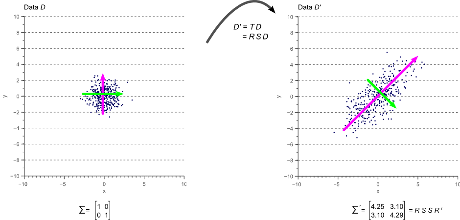
In other words, if we apply the linear transformation defined by ![]() to the original white data
to the original white data ![]() shown by figure 7, we obtain the rotated and scaled data
shown by figure 7, we obtain the rotated and scaled data ![]() with covariance matrix
with covariance matrix ![]() . This is illustrated by figure 10:
. This is illustrated by figure 10:
The colored arrows in figure 10 represent the eigenvectors. The largest eigenvector, i.e. the eigenvector with the largest corresponding eigenvalue, always points in the direction of the largest variance of the data and thereby defines its orientation. Subsequent eigenvectors are always orthogonal to the largest eigenvector due to the orthogonality of rotation matrices.
Conclusion
In this article we showed that the covariance matrix of observed data is directly related to a linear transformation of white, uncorrelated data. This linear transformation is completely defined by the eigenvectors and eigenvalues of the data. While the eigenvectors represent the rotation matrix, the eigenvalues correspond to the square of the scaling factor in each dimension.
If you’re new to this blog, don’t forget to subscribe, or follow me on twitter!




Great article thank you
The covariance matrix is symmetric. Hence we can find a basis of orthonormal eigenvectors and then $\Sigma=VL V^T$.
From computational point of view it is much simpler to find $V^T$ than $V^{-1}$.
Very true, Alex, and thanks for your comment! This is also written in the article: “Furthermore, since R is an orthogonal matrix, R^{-1} = R^T”. But you are right that I only mention this near the end of the article, mostly because it is easier to develop an intuitive understanding of the first part of the article by considering R^{-1} instead of R^T.
Great post! I had a couple questions:
1) The data D doesn’t need to be Gaussian does it?
2) Is [9] reversed (should D be on the left)?
Hi Brian:
1) Indeed the data D does not need to be Gaussian for the theory to hold, I should probably have made that more clear in the article. However, talking about covariance matrices often does not have much meaning in highly non-Gaussian data.
2) That depends on whether D is a row vector or a column vector I suppose. In this case, if each column of D is a data entry, then R*D = (D^t*R)^t
Thank you for this great post! But let me please correct one fundamental mistake that you made. The square root of covariance matrix M is not equal to R * S. The square root of M equals R * S * R’, where R’ is transposed R. Proof: (R * S * R’) * (R * S * R’) = R * S * R’ * R * S * R’ = R * S * S * R’ = T * T’ = M. And, of course, T is not a symmetric matrix (in your post T = T’, which is wrong).
Thanks a lot for noticing! You are right indeed, I will get back about this soon (don’t really have time right now).
Edit: I just fixed this mistake. Sorry for the long delay, I didn’t find the time before. Thanks a lot for your feedback!
Very Useful Article What I feel needs to be included is the interpretation of the action of the covariance matrix as a linear operator. For example, the eigen vectors of the covariance matrix form the principal components in PCA. So, basically , the covariance matrix takes an input data point ( vector ) and if it resembles the data points from which the operator was obtained, it keeps it invariant ( upto scaling ). Is there a better way to interpret the eigenvectors of covariance matrix ?
Hi Kumar, great point! This is basically captured by equations 13 and 14, but I just added a short section to make this a bit more clear in the article.
“..the eigenvectors represent the directions of the largest variance of the data, the eigenvalues represent the magnitude of this variance in those directions..” … Thanks a lot for expressing it so precisely.
Thank you for such an intuitive article. I have spent countless hours over countless days trying to picture exactly what you described. I wonder if you can clarify something in the writing, though. When you first talk about vector v, throughout the entire paragraph, it is referred to both as a unit vector and a vector whose length is set to match the spread of data in the direction of v.
By the way, would you know of a similarly intuitive description of cov(X,Y), where X and Y are disjoint sets of random variables?
Quoting a portion of the text above ” …..we should choose its components such that the covariance matrix \vec{v}^{\intercal} \Sigma \vec{v} of the projected data is as large as possible….”
That quantity “\vec{v}^{\intercal} \Sigma \vec{v}” (sorry – I am not able to do a graphical paste – but I hope you know what I mean) is not a matrix – It is a scalar quantity – isn’t it?
Or what you wanted to say was ” …..we should choose its components such that the covariance of the data with the vector v is as large as possible….”. And this covariance is a term of the Raliegh’s coefficient ……
May be there is a better way to put …
The better way is to say that it is just a variance of projected data. So, that is a mistake, it should be variance, not covariance.
Hello Vincent,
Thank you very much for this blog post. I have one question though concerning figure 4: Shouldn’t the magenta eigenvector in the right part of the picture point downwards? Otherwise, we wouldn’t have a proper rotation.
Best regards,
Lukas
The correlations you showin figure 5 look a lot like Reduced Major Axis. How do do the eigenvectors and RMA compare?. Of course, there is nothing like eigenvalues in the RMA but could they be estimated from the ranges of values after rotation of the RMA regression?
Gordon
I love to reread your articles. Hope to see more such intuitive topics!!!
Great Thank you.
Thanks a lot. Very intuitive articles on the covariance matrix.
Always wondered why Eigen vectors of covariance matrix and the actual data were similar. Thanks for the tutorial. It helped in clearing the doubt.
Great article!!! It’s soooooo helpful, thank you
Thanks for sharing this article, it’s a wonderful read!
Am I correct in understanding that the transformation TT^t for the covariance matrix will apply when transforming any data by T, not just for white data?
Nice article. Thank you so much!
Superb!
It is just awesome that you are so open to suggestions and then make the changes for the benefit of all of us.
Thank You, Thank You, Thank You!!
excellent article. gave me a whole new perspective of covariance matrix.
Thanks man, great article! So useful for my PhD !
Do you know of any mathematics book where I can find a rigorous dissertation about this? My professor wants me to be as meticulous as possible
Thank you in advance!
Do you know of any mathematics book where I can find a rigorous dissertation about this?
education system need people like you
it was really an informative article,thanks a lot
This is a great article, thank you so much! I completely agree with your motivation to write things down in a simple way, rather than trying to sound smart to people who already know everything. I learned so much from your blog in a short time.
Thanks for this! This and the companion eigen decomposition article were exactly what I was looking for, and much easier to understand than other resources I found.
Great text. Good job! Thank you
Great article, but one doubt. It was mentioned that direction of eigen vector remains unchanged when linear transformation is applied. But in Fig. 10, direction of the vector is also changed. Can you please explain it?
Very useful. Thanks!
Very good explain and worthful.
But I have doubt why does eigenvector have one direction even though spread is in both directions.
It’s true that both cancel out and we are left with zero…
Where I am going geometrically worng.
Second
Why don’t we a complex eigen vector conjugate when we rotate the white data by rotational matrix….
Really intuitive write up, it was a joy to read.
In figures 4 and 5, though, the v_i are unit vectors and have norm 1. You want to write var(v_i) instead of norm(v_i) in both those figures, as norm(v_i) = 1 but var(v_i) = λ_i.
Great post! I have one question though. What if some of the eigenvalues are negative? Then how can you decompose L into SS^T
In figure 4. Did you swap the element in the vector
in the Left : I think it should be V1 = [1 0] and V2 = [0 1]
in the Right : I think it should be V1 = [0 1] and V2 = [1 0]
if I missunderstand something im sorry
Very useful article but I faced some errors while implementing this.
I tried to do svd decomposition of the covariance matrix and got L matrix as the square of scaling coefficients(not exactly equal but very close Note:implemented in matlab) but the the Rotation matrix I got weird matrix where the first element in the matrix cos(theta) is negative and last element in the matrix is postive. Here is the code if you want to have a look (https://drive.google.com/open?id=0B0Dif3DoeegwY1NuNlFUVUc4eXFsTGtSeFl4YkFDMXRDWHVj)
Very lucid article. I have a question. If one of the eigenvalues (say lambda) has a multiplicity bigger than 1 (say 2 for simplicity), then, theoretically, one can chose different sets of two eigenvectors associated with lambda. How does that Does that affect the interpretation? This is relevant when one is constructing the principal components that would give most information about the data. Thank for your attention to me question. –ekwaysan
Very useful article. However, I don’t understand how \vec{v}^{\intercal} \Sigma \vec{v} is the variance of the projected data. Can anyone explain it for me?
Thanks in advance!
Thank you a lot.. I was trying to implement my mcmc code using a proposal covariance matrix and thanks to your method everything is clear to me now
Awesome article! Really helped me to understand this eigenvalue/eigenvector stuff :)..thanks!!!
Really cool. I though I would never find the correlation of these matrices and transformations in the CMA-ES algorithm.
very instructive!! thank you-
Great write up and explanation.
Consider \Sigma = [2 0.1; 0.1 3]; If you perform an eigenvalue-eigenvector decomposition, i.e. P = VLV^T. The V obtained is no longer a rotation matrix. It is orthogonal but not a rotation matrix. I think Niranjan Kotha sees the same issue. The problem is that the factorization doesn’t always yield a rotation matrix (orthogonal yes, but not the special orthogonal matrix).
I really liked this explanation, thanks.