The Curse of Dimensionality in classification
Introduction
In this article, we will discuss the so called ‘Curse of Dimensionality’, and explain why it is important when designing a classifier. In the following sections I will provide an intuitive explanation of this concept, illustrated by a clear example of overfitting due to the curse of dimensionality.
Consider an example in which we have a set of images, each of which depicts either a cat or a dog. We would like to create a classifier that is able to distinguish dogs from cats automatically. To do so, we first need to think about a descriptor for each object class that can be expressed by numbers, such that a mathematical algorithm, i.e. a classifier, can use these numbers to recognize the object. We could for instance argue that cats and dogs generally differ in color. A possible descriptor that discriminates these two classes could then consist of three number; the average red color, the average green color and the average blue color of the image under consideration. A simple linear classifier for instance, could combine these features linearly to decide on the class label:
If 0.5*red + 0.3*green + 0.2*blue > 0.6 : return cat;
else return dog;
However, these three color-describing numbers, called features, will obviously not suffice to obtain a perfect classification. Therefore, we could decide to add some features that describe the texture of the image, for instance by calculating the average edge or gradient intensity in both the X and Y direction. We now have 5 features that, in combination, could possibly be used by a classification algorithm to distinguish cats from dogs.
To obtain an even more accurate classification, we could add more features, based on color or texture histograms, statistical moments, etc. Maybe we can obtain a perfect classification by carefully defining a few hundred of these features? The answer to this question might sound a bit counter-intuitive: no we can not!. In fact, after a certain point, increasing the dimensionality of the problem by adding new features would actually degrade the performance of our classifier. This is illustrated by figure 1, and is often referred to as ‘The Curse of Dimensionality’.
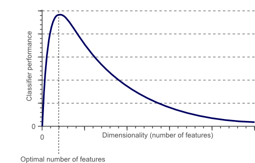
Figure 1. As the dimensionality increases, the classifier’s performance increases until the optimal number of features is reached. Further increasing the dimensionality without increasing the number of training samples results in a decrease in classifier performance.
In the next sections we will review why the above is true, and how the curse of dimensionality can be avoided.
The curse of dimensionality and overfitting
In the earlier introduced example of cats and dogs, let’s assume there are an infinite number of cats and dogs living on our planet. However, due to our limited time and processing power, we were only able to obtain 10 pictures of cats and dogs. The end-goal in classification is then to train a classifier based on these 10 training instances, that is able to correctly classify the infinite number of dog and cat instances which we do not have any information about.
Now let’s use a simple linear classifier and try to obtain a perfect classification. We can start by a single feature, e.g. the average ‘red’ color in the image:
Figure 2 shows that we do not obtain a perfect classification result if only a single feature is used. Therefore, we might decide to add another feature, e.g. the average ‘green’ color in the image:
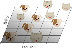
Figure 3.Adding a second feature still does not result in a linearly separable classification problem: No single line can separate all cats from all dogs in this example.
Finally we decide to add a third feature, e.g. the average ‘blue’ color in the image, yielding a three-dimensional feature space:
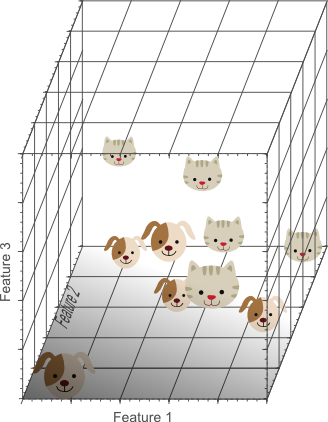
Figure 4. Adding a third feature results in a linearly separable classification problem in our example. A plane exists that perfectly separates dogs from cats.
In the three-dimensional feature space, we can now find a plane that perfectly separates dogs from cats. This means that a linear combination of the three features can be used to obtain perfect classification results on our training data of 10 images:
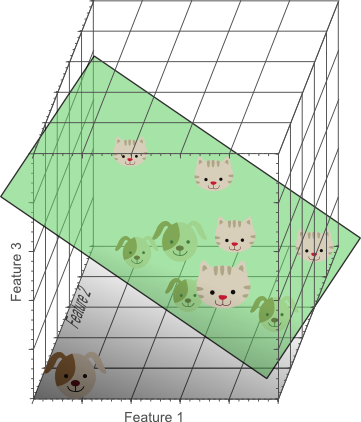
Figure 5. The more features we use, the higher the likelihood that we can successfully separate the classes perfectly.
The above illustrations might seem to suggest that increasing the number of features until perfect classification results are obtained is the best way to train a classifier, whereas in the introduction, illustrated by figure 1, we argued that this is not the case. However, note how the density of the training samples decreased exponentially when we increased the dimensionality of the problem.
In the 1D case (figure 2), 10 training instances covered the complete 1D feature space, the width of which was 5 unit intervals. Therefore, in the 1D case, the sample density was 10/5=2 samples/interval. In the 2D case however (figure 3), we still had 10 training instances at our disposal, which now cover a 2D feature space with an area of 5×5=25 unit squares. Therefore, in the 2D case, the sample density was 10/25 = 0.4 samples/interval. Finally, in the 3D case, the 10 samples had to cover a feature space volume of 5x5x5=125 unit cubes. Therefore, in the 3D case, the sample density was 10/125 = 0.08 samples/interval.
If we would keep adding features, the dimensionality of the feature space grows, and becomes sparser and sparser. Due to this sparsity, it becomes much more easy to find a separable hyperplane because the likelihood that a training sample lies on the wrong side of the best hyperplane becomes infinitely small when the number of features becomes infinitely large. However, if we project the highly dimensional classification result back to a lower dimensional space, a serious problem associated with this approach becomes evident:
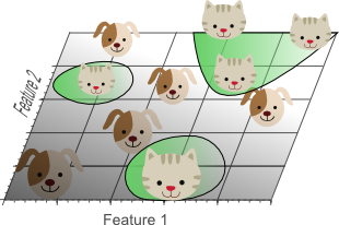
Figure 6. Using too many features results in overfitting. The classifier starts learning exceptions that are specific to the training data and do not generalize well when new data is encountered.
Figure 6 shows the 3D classification results, projected onto a 2D feature space. Whereas the data was linearly separable in the 3D space, this is not the case in a lower dimensional feature space. In fact, adding the third dimension to obtain perfect classification results, simply corresponds to using a complicated non-linear classifier in the lower dimensional feature space. As a result, the classifier learns the appearance of specific instances and exceptions of our training dataset. Because of this, the resulting classifier would fail on real-world data, consisting of an infinite amount of unseen cats and dogs that often do not adhere to these exceptions.
This concept is called overfitting and is a direct result of the curse of dimensionality. Figure 7 shows the result of a linear classifier that has been trained using only 2 features instead of 3:
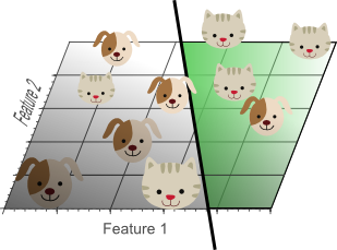
Figure 7. Although the training data is not classified perfectly, this classifier achieves better results on unseen data than the one from figure 5.
Although the simple linear classifier with decision boundaries shown by figure 7 seems to perform worse than the non-linear classifier in figure 5, this simple classifier generalizes much better to unseen data because it did not learn specific exceptions that were only in our training data by coincidence. In other words, by using less features, the curse of dimensionality was avoided such that the classifier did not overfit the training data.
Figure 8 illustrates the above in a different manner. Let’s say we want to train a classifier using only a single feature whose value ranges from 0 to 1. Let’s assume that this feature is unique for each cat and dog. If we want our training data to cover 20% of this range, then the amount of training data needed is 20% of the complete population of cats and dogs. Now, if we add another feature, resulting in a 2D feature space, things change; To cover 20% of the 2D feature range, we now need to obtain 45% of the complete population of cats and dogs in each dimension (0.45^2 = 0.2). In the 3D case this gets even worse: to cover 20% of the 3D feature range, we need to obtain 58% of the population in each dimension (0.58^3 = 0.2).

Figure 8. The amount of training data needed to cover 20% of the feature range grows exponentially with the number of dimensions.
In other words, if the amount of available training data is fixed, then overfitting occurs if we keep adding dimensions. On the other hand, if we keep adding dimensions, the amount of training data needs to grow exponentially fast to maintain the same coverage and to avoid overfitting.
In the above example, we showed that the curse of dimensionality introduces sparseness of the training data. The more features we use, the more sparse the data becomes such that accurate estimation of the classifier’s parameters (i.e. its decision boundaries) becomes more difficult. Another effect of the curse of dimensionality, is that this sparseness is not uniformly distributed over the search space. In fact, data around the origin (at the center of the hypercube) is much more sparse than data in the corners of the search space. This can be understood as follows:
Imagine a unit square that represents the 2D feature space. The average of the feature space is the center of this unit square, and all points within unit distance from this center, are inside a unit circle that inscribes the unit square. The training samples that do not fall within this unit circle are closer to the corners of the search space than to its center. These samples are difficult to classify because their feature values greatly differs (e.g. samples in opposite corners of the unit square). Therefore, classification is easier if most samples fall inside the inscribed unit circle, illustrated by figure 9:
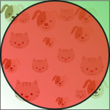
Figure 9.Training samples that fall outside the unit circle are in the corners of the feature space and are more difficult to classify than samples near the center of the feature space.
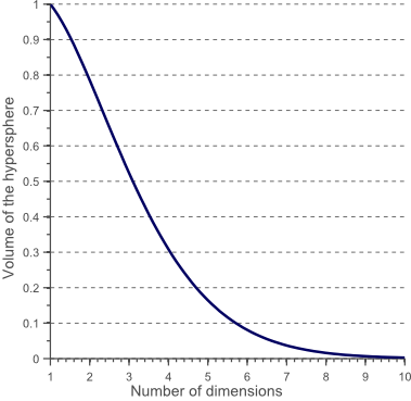
An interesting question is now how the volume of the circle (hypersphere) changes relative to the volume of the square (hypercube) when we increase the dimensionality of the feature space. The volume of a unit hypercube of dimension d is always 1^d = 1. The volume of the inscribing hypersphere of dimension d and with radius 0.5 can be calculated as:
(1) 
Figure 10 shows how the volume of this hypersphere changes when the dimensionality increases:
This shows that the volume of the hypersphere tends to zero as the dimensionality tends to infinity, whereas the volume of the surrounding hypercube remains constant. This surprising and rather counter-intuitive observation partially explains the problems associated with the curse of dimensionality in classification: In high dimensional spaces, most of the training data resides in the corners of the hypercube defining the feature space. As mentioned before, instances in the corners of the feature space are much more difficult to classify than instances around the centroid of the hypersphere. This is illustrated by figure 11, which shows a 2D unit square, a 3D unit cube, and a creative visualization of an 8D hypercube which has 2^8 = 256 corners:
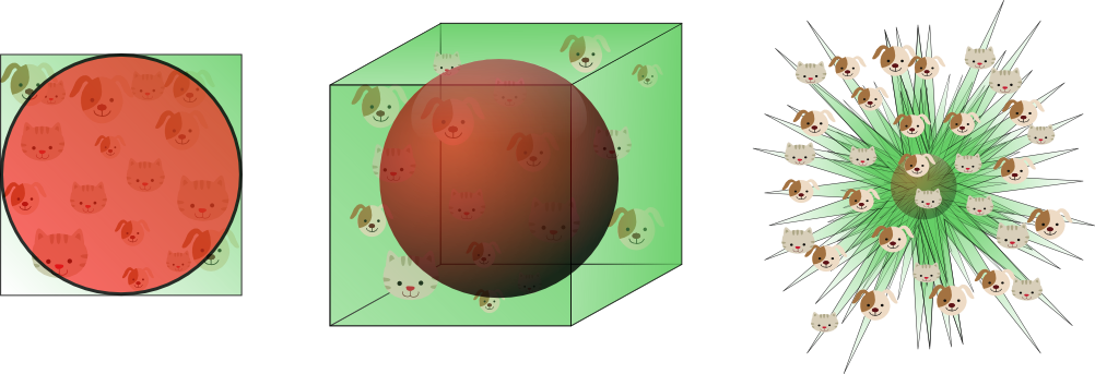
Figure 11. As the dimensionality increases, a larger percentage of the training data resides in the corners of the feature space.
For an 8-dimensional hypercube, about 98% of the data is concentrated in its 256 corners. As a result, when the dimensionality of the feature space goes to infinity, the ratio of the difference in minimum and maximum Euclidean distance from sample point to the centroid, and the minimum distance itself, tends to zero:
(2) ![]()
Therefore, distance measures start losing their effectiveness to measure dissimilarity in highly dimensional spaces. Since classifiers depend on these distance measures (e.g. Euclidean distance, Mahalanobis distance, Manhattan distance), classification is often easier in lower-dimensional spaces where less features are used to describe the object of interest. Similarly, Gaussian likelihoods become flat and heavy tailed distributions in high dimensional spaces, such that the ratio of the difference between the minimum and maximum likelihood and the minimum likelihood itself tends to zero.
How to avoid the curse of dimensionality?
Figure 1 showed that the performance of a classifier decreases when the dimensionality of the problem becomes too large. The question then is what ‘too large’ means, and how overfitting can be avoided. Regrettably there is no fixed rule that defines how many feature should be used in a classification problem. In fact, this depends on the amount of training data available, the complexity of the decision boundaries, and the type of classifier used.
If the theoretical infinite number of training samples would be available, the curse of dimensionality does not apply and we could simply use an infinite number of features to obtain perfect classification. The smaller the size of the training data, the less features should be used. If N training samples suffice to cover a 1D feature space of unit interval size, then N^2 samples are needed to cover a 2D feature space with the same density, and N^3 samples are needed in a 3D feature space. In other words, the number of training instances needed grows exponentially with the number of dimensions used.
Furthermore, classifiers that tend to model non-linear decision boundaries very accurately (e.g. neural networks, KNN classifiers, decision trees) do not generalize well and are prone to overfitting. Therefore, the dimensionality should be kept relatively low when these classifiers are used. If a classifier is used that generalizes easily (e.g. naive Bayesian, linear classifier), then the number of used features can be higher since the classifier itself is less expressive. Figure 6 showed that using a simple classifier model in a high dimensional space corresponds to using a complex classifier model in a lower dimensional space.
Therefore, overfitting occurs both when estimating relatively few parameters in a highly dimensional space, and when estimating a lot of parameters in a lower dimensional space. As an example, consider a Gaussian density function, parameterized by its mean and covariance matrix. Let’s say we operate in a 3D space, such that the covariance matrix is a 3×3 symmetric matrix consisting of 6 unique elements (3 variances on the diagonal and 3 covariances off-diagonal). Together with the 3D mean of the distribution this means that we need to estimate 9 parameters based on our training data, to obtain the Gaussian density that represent the likelihood of our data. In the 1D case, only 2 parameters need to be estimated (mean and variance), whereas in the 2D case 5 parameters are needed (2D mean, two variances and a covariance). Again we can see that the number of parameters to be estimated grows quadratic with the number of dimensions.
In an earlier article we showed that the variance of a parameter estimate increases if the number of parameters to be estimated increases (and if the bias of the estimate and the amount of training data are kept constant). This means that the quality of our parameter estimates decreases if the dimensionality goes up, due to the increase of variance. An increase of classifier variance corresponds to overfitting.
Another interesting question is which features should be used. Given a set of N features; how do we select an optimal subset of M features such that M<N? One approach would be to search for the optimum in the curve shown by figure 1. Since it is often intractable to train and test classifiers for all possible combinations of all features, several methods exist that try to find this optimum in different manners. These methods are called feature selection algorithms and often employ heuristics (greedy methods, best-first methods, etc.) to locate the optimal number and combination of features.
Another approach would be to replace the set of N features by a set of M features, each of which is a combination of the original feature values. Algorithms that try to find the optimal linear or non-linear combination of original features to reduce the dimensionality of the final problem are called Feature Extraction methods. A well known dimensionality reduction technique that yields uncorrelated, linear combinations of the original N features is Principal Component Analysis (PCA). PCA tries to find a linear subspace of lower dimensionality, such that the largest variance of the original data is kept. However, note that the largest variance of the data not necessarily represents the most discriminative information.
Finally, an invaluable technique used to detect and avoid overfitting during classifier training is cross-validation. Cross validation approaches split the original training data into one or more training subsets. During classifier training, one subset is used to test the accuracy and precision of the resulting classifier, while the others are used for parameter estimation. If the classification results on the subsets used for training greatly differ from the results on the subset used for testing, overfitting is in play. Several types of cross-validation such as k-fold cross-validation and leave-one-out cross-validation can be used if only a limited amount of training data is available.
Conclusion
In this article we discussed the importance of feature selection, feature extraction, and cross-validation, in order to avoid overfitting due to the curse of dimensionality. Using a simple example, we reviewed an important effect of the curse of dimensionality in classifier training, namely overfitting.
If you’re new to this blog, don’t forget to subscribe, or follow me on twitter!




Great post, helps me understand this problem much deeper, thanks. Expect more posts from you
Thanks! More posts will follow I’m trying to lay out some basics in my first few posts such that I can start discussing more interesting topics (object tracking, detection in video, etc.) in the near future.
cats! and dogs! ❤ ML
In that case: http://www.wired.com/2012/06/google-x-neural-network/
Really nice article, very informative and well exposed. One thing in the usual argumentation regarding the cod that always leaves me wondering, is that for the curse to strike, the process of raising the dimensionality has to be such, that the data points are equally scattered around in the higher space. I’m not sure this is valid for all cases. Isn’t it so, that more often than not high dimensional problems live in a lower dimensional embedded manifold? This would mean that not every increase in dimensionality introduces necessarily more sparsity in the data. Do you know of any examination in this direction you could point me to?
That’s definitely food for thought, tnx! Intuitively I would say that an increase in dimensionality always increases sparsity in the data due to the fact that the difference between the largest and smallest Euclidean distances between samples in such space becomes indiscernible as the dimensionality grows (figure 11 and equation (1)). Obviously, increased sparsity is not necessarily a bad thing, if the added dimension contributes to the constrast between the different classes. Anyway, I’m not completely sure how to answer your question right now, but I’m going to think about it for a while, thanks. (Feel free to elaborate)
My intuition is that in such a case, you can simply eliminate features that have no discriminatory powers.
Hello, I especially like the graphics you use to make you points clearer. How do you prepare such informative visuals?
Thanks, Anon! My plots are generally created using Matlab, and some external packages (http://www.mathworks.com/matlabcentral/fileexchange/7501-printeps, http://www.mathworks.com/matlabcentral/fileexchange/17928-fixpslinestyle). The other figures are simply drawn in Inscape.
Nice article, but your parameter counting for the Gaussian distribution seems to be off. In 3D the mean would be a vector with 3 parameters, so a total of 9 parameters when you add the 6 parameters from the covariance matrix.
Thanks, Bill! Fixed it.
By the way, the mean for the 2D Gaussian case would have 2 parameters. Also, the sentence that follows the description of fitting a Gaussian (“Again we can see that the number of parameters to be estimated grows exponentially with the number of dimensions.”) is not right — the growth is quadratic.
Obviously you are right. Fixed it, tnx!
leave-on-out cross-validation should be leave-one-out cross-validation
Well spotted I just fixed this typo, tnx!
Very nice article! I just started studying ML and classifiers and this explanation is much clearer than other sources (thanks to the images).
There’s a typo in the Figure 8 paragraph: “using online a single feature”
Tnx for that! I just fixed it.
A well-written and nicely illustrated article! I have some nitpicks though:
1. You can ‘see’ a non-linear classification boundary, as in Fig 6, on a lower dimension when your higher dimensions are functions of your lower dimension. For ex your original dimensions are x1 and x2, and you use a new additional dimension x3 = x1x2. If x3 is an entirely new dimension, then the non-linearity in the lower dimensions may or may not be visible. For ex, with x3, lets say you end up with this classification hyperplane: 2.x1+4.x2+7.x3=10. Projected onto two dimensions this is still a line (at x3=0): 2.x1+4.x2=10
2. Samples falling in different corners of the square are not necessarily difficult to classify – what if different corners are occupied by points with different labels? This is actually a favorable scenario. The other reason you provide is the correct one – given a point in high dimensions, the relative distance between points far from it and close it becomes negligible. Since every classifier (at least the metric classifiers) implicitly or explicitly relies on nearness of correctly labeled points, this is a problem.
Great comment, tnx!
Your first point actually stresses the importance of something I did not address yet in this article (this will be part of a next article): The curse of dimensionality strikes hard if your features are statistically dependent. Indeed in case they are independent (or simply uncorrelated in the Gaussian case), linearity is preserved when projected onto a linear subspace. Regrettably, features are rarely independent.
Thank you for your response!
What matters is whether we know the exact functional relationship of a dimension, x3, to others. Or, can conveniently determine it.
Take a real-world modeling scenario where a feature “location” becomes available for user you want to model. “location” may not entirely be independent of another feature like the “ISP” the user uses for accessing internet. Typically, you wont be determining ‘f’ where ‘location = f(ISP)’. You would be more interested in solving the original classification problem.
Here, if you are looking at hyperplane as a classifier in the new space (i.e. one with location), the projection onto the original space would be a line.
The case that you are talking about is something that, again typically :), a classifier does internally by fabricating new dimensions (basis functions). These can be drawn in the original space to observe the non-linearity.
Vincent –
Thank you so much for putting the effort and time into writing this post! You did an excellent job. Although I’m not new to ML, there is something about the way you explained everything that just sort of ties together everything I know about dimensionality.
You’ve really done a good job, and I’m very thankful that I discovered your blog!
Good luck in your work, and I’m looking forward to reading all of your posts.
Please write more when you can!
Thank you for your kinds words, Bryan! More articles will follow. The first few articles cover the basics of machine learning. I’m hoping to progress soon to more interesting and practical articles about object detection and tracking in video.
Have you checked the curse of big data? (http://www.analyticbridge.com/profiles/blogs/the-curse-of-big-data)
Interesting article, tnx! A nice demonstration about this is: http://www.tylervigen.com/
This is simply the best explanation Ive found of the “The curse of dimensionality”. Thanks and please keep writing clearly like this forever!
Thank you, Julio! I’ll most definitely try to keep up the pace
thanks for your intuitive explanation about the curse of dimensionality. heard of the issue many times roughly but didn’t find anything as thorough and informative as this article. thank u for your sharing.
Thanks a lot for these encouraging words!
Very inspiring. I like the way you argumented. But one think is still not really clear. That is the argument about the distance (formula 2). It is nearly the same statement as in Wikipedia, where it is also unclear, how the distances are related to the dimensions and how this argument implies that the distances become use less.
Hi Thomas, tnx for commenting! Basically, it can be shown that in high dimensional spaces, the ratio of the distances of the nearest and farthest neighbors of a data point tends to 1. This means that the concept of proximity (especially under the L2 norm) becomes meaningless. Interesting reads on this topic are http://www.researchgate.net/publication/30013021_On_the_Surprising_Behavior_of_Distance_Metric_in_High-Dimensional_Space/file/e0b49525c3e5ba1720.pdf and http://web.cs.sunyit.edu/~mike/cs542/nearestneighbormeaningful.pdf
Wow, this is super interesting! Just came upon your article from a stackexchange post, and I love your intuitive explanation of the curse of dimensionality; great work!
Hi Vincent,
you should be careful concerning this statement, since the authors of the original article (which I read in the meantime) state, that “under a certain precondition” this statement holds.
This precondition says that “the variance of the distance distribution scaled by the overall magnitudes of the distances converges to 0″,which is true only for certain types of data distributions and dimensions types. E.g. it is fulfilled for IID (independent and identical distributed dimensions) like independent random data uniformly distributed in every dimension). That’s an example of one extrem distribution. But it is not fulfilled for data distributed on a “hyperline” where the values of the data points in all dimensions are equal. That’s another extrem distribution.
Hence – and that is the real interesting part of the proof – whether the distance function looses it’s meaning depends not on the particular distance function used, but instead on the structure of distributions of the n-dimensions (whether all features have an identical distribution, depend on each other or are non-identically distributed) and the data distributions themselfs (whether they are independent or not, uniformly distributed or tend to form clusters).
So, whether this argument is relevant for a learning problem, needs always be discussed in the light of the particular feature distributions, the data and especially the behaviour of the variances.
Anyway thanx, for pushing me to read the original paper, since this insight is much more worth than unconditioned statement of formula 2.
That’s a great point, Thomas, and indeed you are right! Tnx a lot for your feedback and for summarizing the paper mentioned. I will change the article to include this one of these days (don’t have time now).
[…] you are not yet familiar with this approach and its immanent problems of overfitting, etc. read “The Curse of Dimensionality in classification”). However, as we keep increasing dimensions, the computational cost of measuring the similiarity […]
Hello, in your comment about cross validation, i think you should make it more clear. In k fold, The data is broken up into a number of equal subsets. one subset is chosen as the test data, the remaining subsets are used for training. Since you used the word “other” subsets, I think the way you described it could be misinterpreted as train on one subset, test on the remaining, ..which isn’t what this wiki article suggests http://en.wikipedia.org/wiki/Cross-validation_%28statistics%29#k-fold_cross-validation but nice post anyway.
Tnx for your comment Aaron, and you are right! I updated the paragraph accordingly.
Hi Vincent,
Thanks a lot for this. It’s a great explanation of what the dangers are of overfitting.
However, I wonder why you propose PCA as a good method to counter overfitting because you said yourself: “However, note that the largest variance of the data not necessarily represents the most discriminative information.”? Isn’t it much better to add regularization in your model? I understand that the article would become a bit too long if that needs to be explained as well, but I think it’s better than suggesting PCA as a good technique to reduce overfitting.
Hi Jonas, good point! The reason I introduce PCA here is because it is one of the most widely used dimensionality reduction techniques, so the topic is definitely relevant to those interested in the curse of dimensionality. In very high dimensional settings, PCA can almost always be used to fight the curse of dimensionality. In the article, I linked to another article of mine, about PCA (http://www.visiondummy.com/2014/05/feature-extraction-using-pca/) where its shortcomings are discussed in more detail, and other techniques such as LDA are proposed. Nevertheless, regularization is always important to avoid overfitting your models, whether or not you use feature extraction and selection techniques, even in low dimensional settings. However, regularization itself is a huge research domain and deserves an article on its own. I promise you that I’ll write one about this soon :).
Thanks for the excellent posts! These are very helpful.
I’m really interested in the topic of generalization, and the differences between linear and nonlinear classifiers that you allude to. Any chance you could write a post that focuses on generalization and/or the linear/non-linear issue?
Awesome, just loved it. Very simple explanation with examples.
Really well explained Vincent – thanks for your post.
Thank you for the post! Have looked through several academic articles on the topic, your explanation is the best!
Excellent. Thanks Vincent. Btw, I shared the article on Twitter
I’m confused about the illustration of Figure 9:Training samples that fall outside the unit circle are in the corners of the feature space and are more difficult to classify than samples near the center of the feature space.
Why are the samples near the center easier to classify?
And why are the samples in the corners more difficult to classify?
Can we have pdf version of these pages as well? Really helpful
I’ve searched and searched and this was THE best explanation I found online. Thanks so much for this!
Article is informative but I am confused how to find optimal number of dimensions for dimension reduction techniques?
Hi, can you please explain what does the ratio dmax-dmin/dmin represents, why does it goes to zero and what does it mean? why is the distance from the center related to distance to neighbours if one would consider a KNN classifier in high dimension?
Hi Vincent,
Thanks a lot for this useful Article. It’s a great explanation of (curse of Dimensionality).
I am interested in the first figure which shows the relation between the number of dimensions and classifier performance.
Is it possible to provide me some references that provide this figure with more details and experimental result, or any reference that contain this figure.
I suggest, it would be useful if you show the references that you used in writing your articles on this site.
Thanks in advance for answering or providing any reference.
Well written topic Vincent,good job.
However can you explain briefly (or confirm if it is true): Is the unitary hypershpere realated to clustering because clastering uses the Euclidean distance from the center?
Thank you for your time
Hi Vincent, first of all I would like to thank you for the wonder blog post and the work you are doing on visiondummy.
I had one doubt about equation 2. Shouldn’t there be only one distance from a sample point to a centroid? How can there be two distances i.e minimum and maximum distances?
Hi, I am a student who follows data analytics course module I my university. I was so confused with all the theories and awful explanations by the lecturer. Thank god I found this article!